TR-by-TR Cue-locked Timeseries
The masked_timeseries module extracts timeseries for region of interest (ROI) mask or ROI coordinates and generates TR-by-TR cue-locked timeseries. Below I cover three primary functions: extract_time_series extract_postcue_trs_for_conditions and plot_responses functions. extract_time_series extracts the values from BOLD files, extract_postcue_trs_for_conditions aligns events timings to TRs ans generates TR-by-TR values and plot_responses uses the resulting values to generate a TR-by-TR figure.
extract_time_series
As mentioned above, the extract_time_series function extracts time series data from BOLD images for specified ROI or coordinates. This is achieve by either using NiftiLabelsMasker or nifti_spheres_masker from Nilearn to extract the timeseries and average the voxels within that ROI.
extract_time_series
As mentioned above, the extract_time_series function extracts time series data from BOLD images for specified regions of interest (ROI) or coordinates. The function uses either NiftiLabelsMasker or NiftiSpheresMasker from Nilearn to perform the extraction.
- To use the extract_time_series function, you have to provide the following information:
bold_paths: A list of paths to the BOLD image files for each subject, run, and/or session.
roi_type: The type of ROI (‘mask’ or ‘coords’).
high_pass_sec: The high-pass filter cutoff in seconds (optional).
roi_mask: The path to the ROI mask file. If this is provided, the function will use NiftiLabelsMasker (required if roi_type is ‘mask’).
roi_coords: A tuple of coordinates (x, y, z) for the center of the sphere ROI (required if roi_type is ‘coords’).
radius_mm: The radius of the sphere in millimeters (required if roi_type is ‘coords’).
detrend: Whether to detrend the BOLD signal using Nilearn’s detrend function (optional, default is False).
fwhm_smooth: The full-width at half-maximum (FWHM) value for Gaussian smoothing of the BOLD data (optional).
n_jobs: The number of CPUs to use for parallel processing (optional, default is 1). Depending on data size, at least 16GB per CPU is recommended.
- The function returns:
- If roi_type is ‘mask’:
List of numpy arrays containing the extracted time series data for each subject/run.
List of subject information strings formatted as ‘sub-{sub_id}_run-{run_id}’ reflecting the order of list of timeseries arrays.
- If roi_type is ‘coords’:
List of numpy arrays containing the extracted time series data for each subject/run.
Nifti1Image coordinate mask that was used in the timeseries extraction.
List of subject information strings formatted as ‘sub-{sub_id}_run-{run_id}’ reflecting the order of list of timeseries arrays.
Utility
Simply, in fMRI, the goal is to fit a design matrix (comprised of task-relevant stimulus onsets & nuisance regressors), \(X\beta\), to timeseries data, \(Y\), for every given voxel or ROI. Plus some noise, \(\epsilon\). The model being:
A whole brain scan can can comprised of hundreds of thousands of voxels. However, we can use an ROI mask to get the average of voxels for a given mask for each volume (t). Any example of what that may look like from the AHRB study:
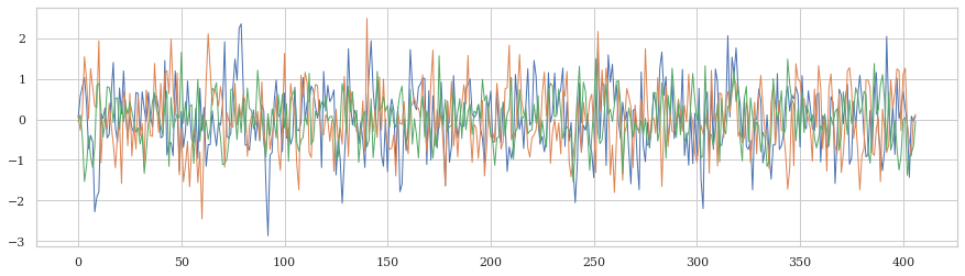
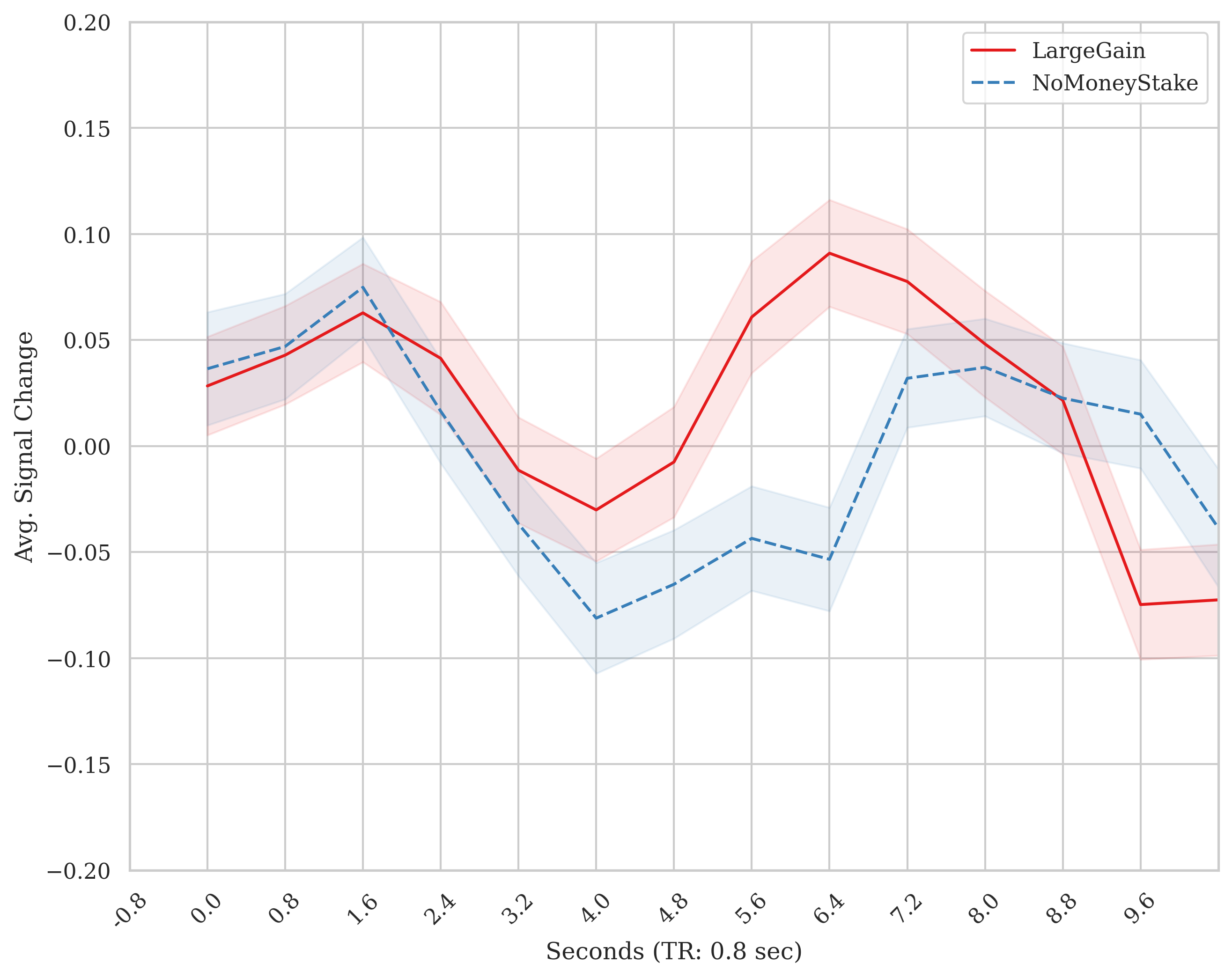
In the timeseries, there is a lot of variability. It is also harder to see meaningful fluctuations because we 1) can’t easily see when events occur and 2) the change in amplitude is often very small. See discussions in Drew (2019) and Drew (2022). Nevertheless, by plotting the data for a given ROI/voxel, you can observe the change. Below is an example of how locked the onset of two cues, LargeGain and NoMoneyStake to the TRs from the timeseries from a modified version of the MID task, a change may be observed.
The purpose of the masked_timeseries.py module is to perform this sort of data extraction and plotting. Often, it is useful to dump out your timeseries signal to confirm that you are getting a response in visual and/or motor regions around the times they should occur. Second to the large effect regions, evaluating whether you are observed a response in a ROI specific to the process/stimulus of interest.
Example
dummy exampple Let’s start off with a conceptual example. Say you have a time series for cue evoked response: Happy & Sad photos. You extract timeseries for a region that is more sensitive to Happy > Sad (whatever that may be…). In this region, these two cues would be differentiated by the signal. A prior, there is a thesis for how this may be. First, take a peak at the fake timeseries that includes both events.
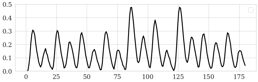
It is a bit challenging to make out which even is where. Let’s add sticks at which time the events occur.
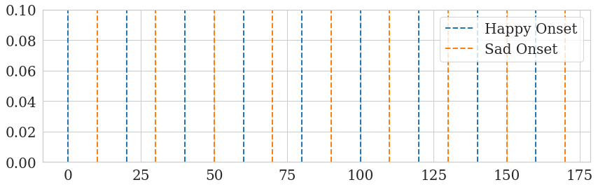
Now, let’s combine the two to see how the fake BOLD response is delayed after each cue but follows some ordered structure. The trend of the data becomes more apparent.
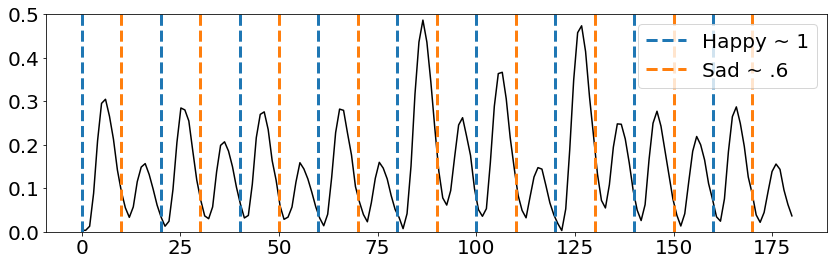
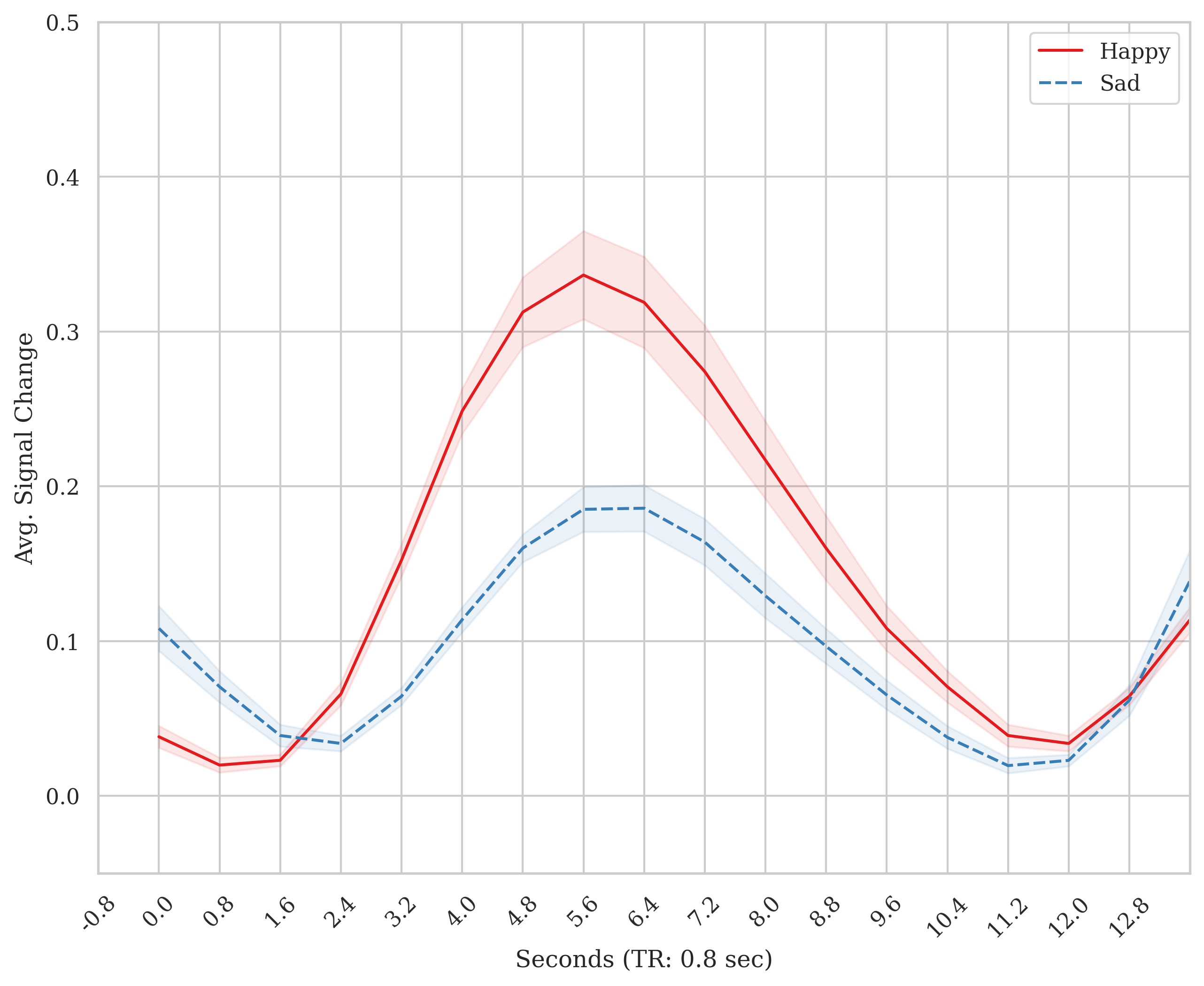
In this example, the the effect for Happy was intentionally made larger than Sad. So it is easier to visualize as it is made with Nilearn’s SPM function (for code of this end-to-end example, see end of this doc). Nevertheless, we can extract the timeseries locked to these conditions to make it especially apparent:
masked_timeseries example Now, I will review an example of how timeseries for an ROI can be extracted, locked to event files and plotted TR-by-TR using the masked_timeseries.py module.
from pyrelimri import masked_timeseries

n3_boldpaths = ["./sub-1-ses-1_task-kewl_run-01_bold.nii.gz", "./sub-2-ses-1_task-kewl_run-01_bold.nii.gz", "./sub-3-ses-1_task-kewl_run-01_bold.nii.gz"]
roi_mask_path = "./roi_mask.nii.gz"

# mask versus coordinates example
timeser_mask_n3, id_order = masked_timeseries.extract_time_series(bold_paths=n3_boldpaths, roi_type='mask',
                                                                  high_pass_sec=True, roi_mask=roi_mask_path,
                                                                  detrend=True, fwhm_smooth=4, n_jobs=2)
# Extract timeseries using ROI coordinates with a radius of 6mm
# coordinates
coords = [(30, -22, -18), (50, 30, 40)]
timeser_coord_n3, roi_sphere, id_order = masked_timeseries.extract_time_series(masked_timeseries.extract_time_series(bold_paths=n3_boldpaths,
                                                                                                                  roi_type='coords', high_pass_sec=True,
                                                                                                                  roi_coords=coords, radius_mm=6,
                                                                                                               detrend=True, fwhm_smooth=4, n_jobs=2)
extract_postcue_trs_for_conditions
This function extracts the TR-by-TR cue-locked timeseries for different conditions at cue onset + TR delay.
- To use the extract_postcue_trs_for_conditions function, you have to provide the following information:
events_data: A list of paths to the behavioral data files. This should match the order of subjects/runs/tasks as the BOLD file list.
onset: The name of the column containing onset values in the behavioral data.
trial_name: The name of the column containing condition values in the behavioral data.
bold_tr: The repetition time (TR) for the acquisition of BOLD data in seconds.
bold_vols: The number of volumes for BOLD acquisition.
time_series: The timeseries data extracted using the extract_time_series function.
conditions: A list of conditions to extract the post-cue timeseries for.
tr_delay: The number of TRs after onset of stimulus to extract and plot.
list_trpaths: The list of subject information strings formatted as ‘sub-{sub_id}_run-{run_id}’.
The function returns a pandas DataFrame containing mean signal intensity values, subject labels, trial labels, TR values, and cue labels for all specified conditions.
Example:
from pyrelimri import masked_timeseries

# Paths to events files
events_data = ['/sub-1-ses-1_task-kewl_run-01_events.csv', './sub-2-ses-1_task-kewl_run-01_events.csv', './sub-3-ses-1_task-kewl_run-01_events.csv']

# Onset column name
onset = 'onset'

# Trial type column name for onset timees and conditions, and list of conditions to plot
trial_name = 'trial_type'
conditions = ['Happy', 'Sad']

# TR delay, 0 + delay to create
tr_delay = 5

# Extract post-cue timeseries for conditions. Notice, timeser_mask_n3 and id_order are from above example
out_df = masked_timeseries.extract_postcue_trs_for_conditions(
    events_data=events_data, onset=onset, trial_name=trial_name, bold_tr=2.0, bold_vols=150,
    time_series=timeser_mask_n3, conditions=conditions, tr_delay=12, list_trpaths=id_order
)
plot_responses
This function plots the average response for each condition using the post-cue timeseries.
- To use the plot_responses function, you need to provide:
postcue_timeseries_dict: The dictionary with post-cue timeseries for each condition.
conditions: The list of conditions to plot.
output_file: The path to save the plot image.
The function does not return any value, but it saves the plot to the specified output file.
Example:
# Path to save the plot image
output_file = "./responses_plot.png"

# Plot average responses for conditions
masked_timeseries.plot_responses(postcue_timeseries_dict=out_df, conditions=conditions, output_file=output_file)
This will generate and save a plot of the average response for each condition to the specified output file.
Fake TR-by-TR code
Defined a couple of functions. Some functions from masked_timeseries.py and some functions are based on Russ Poldrack’s MID simulations
def extract_postcue_trs_for_conditions(events_data: list, onset: str, trial_name: str,
                                   bold_tr: float, bold_vols: int, time_series: np.ndarray,
                                   conditions: list, tr_delay: int, list_trpaths: list):

dfs = []
id_list = []
# check array names first
for beh_path in events_data:
    # create sub ID array to text again bold array
    beh_name = os.path.basename(beh_path)
    path_parts = beh_name.split('_')
    sub_id, run_id = None, None
    for val in path_parts:
        if 'sub-' in val:
            sub_id = val.split('-')[1]
        elif 'run-' in val:
            run_id = val.split('-')[1]
    sub_info = 'sub-' + sub_id + '_' + 'run-' + run_id
    id_list.append(sub_info)

assert len(id_list) == len(list_trpaths), f"Length of behavioral files {len(id_list)} does not TR list {len(list_trpaths)}"
assert (np.array(id_list) == np.array(list_trpaths)).all(), "Mismatch in order of IDs between Beh/BOLD"

for cue in conditions:
    cue_dfs = [] # creating separate cue dfs to accomodate different number of trials for cue types
    sub_n = 0
    for index, beh_path in enumerate(events_data):
        subset_df = trlocked_events(events_path=beh_path, onsets_column=onset,
                                    trial_name=trial_name, bold_tr=bold_tr, bold_vols=bold_vols, separator='\t')
        trial_type = subset_df[subset_df[trial_name] == cue]
        out_trs_array = extract_time_series_values(behave_df=trial_type, time_series_array=time_series[index],
                                                   delay=tr_delay)
        sub_n = sub_n + 1  # subject is equated to every event file N, subj n = 1 to len(events_data)

        # nth trial, list of TRs
        for n_trial, trs in enumerate(out_trs_array):
            num_delay = len(trs)  # Number of TRs for the current trial
            if num_delay != tr_delay:
                raise ValueError(f"Mismatch between tr_delay ({tr_delay}) and number of delay TRs ({num_delay})")

            reshaped_array = np.array(trs).reshape(-1, 1)
            df = pd.DataFrame(reshaped_array, columns=['Mean_Signal'])
            df['Subject'] = sub_n
            df['Trial'] = n_trial + 1
            tr_values = np.arange(1, tr_delay + 1)
            df['TR'] = tr_values
            cue_values = [cue] * num_delay
            df['Cue'] = cue_values
            cue_dfs.append(df)

    dfs.append(pd.concat(cue_dfs, ignore_index=True))

return pd.concat(dfs, ignore_index=True)


def plot_responses(df, tr: int, delay: int, style: str = 'white', save_path: str = None,
                   show_plot: bool = True, ylim: tuple = (-1, 1)):

    plt.figure(figsize=(10, 8), dpi=300)
    if style not in ['white', 'whitegrid']:
        raise ValueError("Style should be white or whitegrid, provided:", style)

    sns.set(style=style, font='DejaVu Serif')

    sns.lineplot(x="TR", y="Mean_Signal", hue="Cue", style="Cue", palette="Set1",
                 errorbar='se', err_style="band", err_kws={'alpha': 0.1}, n_boot=1000,
                 legend="brief", data=df)

    if plt_hrf in ['spm','glover']:
        if plt_hrf == 'spm':
            hrf = spm_hrf(tr=tr, oversampling=1, time_length=delay*2, onset=0)
            time_points = np.arange(1, delay + 1, 1)
            plt.plot(time_points, hrf, linewidth=2, linestyle='--',label='SPM HRF', color='black')
        if plt_hrf == 'glover':
            hrf = glover_hrf(tr=tr, oversampling=1, time_length=delay*2, onset=0)
            time_points = np.arange(1, delay + 1, 1)
            plt.plot(time_points, hrf, linewidth=2, linestyle='--',label='Glover HRF', color='black')

    # Set labels and title
    plt.xlabel(f'Seconds (TR: {tr} sec)')
    plt.ylabel('Avg. Signal Change')
    plt.ylim(ylim[0], ylim[1])
    plt.xlim(0, delay)
    plt.xticks(np.arange(0, delay, 1),
               [f'{round((i * tr)-tr, 1)}' for i in range(0, delay)],
               rotation=45)

    # Show legend
    plt.legend(loc='upper right')

    # Check if save_path is provided
    if save_path:
        # Get the directory path from save_path
        directory = os.path.dirname(save_path)
        # Check if directory exists, if not, create it
        if not os.path.exists(directory):
            os.makedirs(directory)
        # Save plot
        plt.savefig(save_path)

    # Show plot if show_plot is True
    if not show_plot:
        plt.close()


def make_stick_function(onsets, durations, length=.1, resolution=.1):
"""
Create a stick function with onsets and durations

Parameters
----------
onsets : list
    List of onset times
durations : list
    List of duration times
length : float
    Length of the stick function (in seconds)
resolution : float
    Resolution of the stick function (in seconds)
    0.1 secs by default

Returns
-------
sf : np.array
    Timepoints of the stick function
"""
timepoints = np.arange(0, length, resolution)
df = np.zeros_like(timepoints)
for onset, duration in zip(onsets, durations):
    df[(timepoints >= onset) & (timepoints < onset + duration)] = 1
sf_df = pd.DataFrame({'impulse': df})
sf_df.index = timepoints
return sf_df

def generate_data(desmtx_conv, beta_dict, noise_sd=.005, beta_sub_sd=.005):
    """
    Generate data based on the design matrix and beta values

    Parameters
    ----------

    desmtx_conv : pd.DataFrame
        Design matrix with convolved regressors
    beta_dict : dict
        Dictionary of beta values for each regressor of interest
    noise_sd : float
        Standard deviation of the noise
    beta_sub_sd : float
        Standard deviation of the betas across subjects
    """
    # check the beta dict
    betas = np.zeros(desmtx_conv.shape[1])
    for key in beta_dict.keys():
        assert key in desmtx_conv.columns, f'{key} not in desmtx'
    betas = np.array([beta_dict[key] if key in beta_dict.keys() else 0 for key in desmtx_conv.columns ], dtype='float32')
    if beta_sub_sd > 0:
        betas += np.random.normal(0, beta_sub_sd, betas.shape)

    data = np.dot(desmtx_conv.values, betas) + np.random.normal(0, noise_sd, desmtx_conv.shape[0])
    data_df = pd.DataFrame({'data': data})
    data_df.index = desmtx_conv.index
    return data_df

def create_conv_mat(eventsdf, tr_dur=None, acq_dur=None):
    vol_time = acq_dur
    tr = tr_dur
    design_mat = make_first_level_design_matrix(
        frame_times=np.linspace(0, vol_time, int(vol_time/tr)),
        events=eventsdf, hrf_model='spm',
        drift_model=None, high_pass=None)
    return design_mat
Create a fake events file, convolve them using Nilearn’s function and generate a timeseries.
task_time = 180
onsets = np.arange(0, task_time, 10)

np.random.seed(11)
dur_opts = [1.5, 2, 2.5]
prob_durs = [.50, .25, .25]
durations = np.random.choice(dur_opts, size=len(onsets), p=prob_durs)

trial_types = ["Happy" if i % 2 == 0 else "Sad" for i in range(len(onsets))]

events_df = pd.DataFrame({
    "onset": onsets,
    "duration": durations,
    "trial_type": trial_types
})

conv_vals = create_conv_mat(eventsdf=events_df, tr_dur=tr, acq_dur=task_time)

beta_dict = {'Happy': 1, 'Sad': .6}
data_fake = generate_data(conv_vals[['Happy','Sad']], beta_dict)
Plot the 1) fake timeseries and 2) timeseries and events combined
plt.figure(figsize=(14, 4))
plt.plot(data_fake, color='black', linewidth=3)
plt.ylim(0,.5)
plt.xticks(fontsize=20)
plt.yticks(fontsize=20)
plt.legend(fontsize=20)
plt.figure(figsize=(14, 4))
plt.plot(data_fake, color='black')
# sticks at each onset
for onset in events_df[events_df['trial_type'] == 'Happy']['onset']:
    plt.vlines(onset, ymin=0, ymax=conv_vals.values.max(), color='#1f77b4', linestyle='--',
               linewidth=3, label='MakinIt ~ 1')

for onset in events_df[events_df['trial_type'] == 'Sad']['onset']:
    plt.vlines(onset, ymin=0, ymax=conv_vals.values.max(), color='#ff7f0e', linestyle='--',
               linewidth=3, label='FakinIt ~ .6')

# only getting main legends
handles, labels = plt.gca().get_legend_handles_labels()
by_label = dict(zip(labels, handles))
plt.legend(by_label.values(), by_label.keys(), fontsize=20)
plt.ylim(0,.5)
plt.xticks(fontsize=20)
plt.yticks(fontsize=20)

plt.show()
First, reshape file from volumes (225, 1) –> into the shape that is expected: number of subjects, volumes, 1 (1, 225, 1). Save the fake events file path for this one fake subject and use it in the function from masked_timeseries.py.
timeseries_reshaped = np.reshape(data_fake, (1, len(data_fake), 1))
events_df.to_csv('/tmp/sub-01_run-01_test-events.csv',sep = '\t')
events_file = ['/tmp/sub-01_run-01_test-events.csv']

events_file = ['/tmp/sub-01_run-01_test-events.csv']
conditions=['Happy','Sad']
trdelay=int(15/tr)
df = extract_postcue_trs_for_conditions(events_data=events_file, onset='onset', trial_name='trial_type',
                                       bold_tr=tr, bold_vols=len(timeseries_reshaped[0]), time_series=timeseries_reshaped,
                                       conditions=conditions, tr_delay=trdelay,list_trpaths=['sub-01_run-01'])
plot_responses(df=df,tr=tr, delay=trdelay, save_path=None,style='whitegrid',
                   show_plot=True, ylim=(-.05, .5))