PyReliMRI Usage
The pyrelimri package contains multiple modules for calculating image reliability measures.
brain_icc
From pyrelimri, the brain_icc module contains functions for voxelwise and atlas-based intraclass correlation estimates on 3D volumes.
voxelwise_icc
- pyrelimri.brain_icc.voxelwise_icc(multisession_list: list, mask: str, icc_type: str = 'icc_3', n_jobs: int = -1) dict[source]
Calculate the Intraclass Correlation Coefficient (ICC) along with lower and upper bound confidence intervals by voxel for specified input files using manual sum of squares calculations. Now parallelized!
- Parameters:
multisession_list (list of list of str) –
List of lists containing paths to subject 3D volumes for each session.
Example
dat_ses1 = [“./ses1/sub-00_Contrast-A_bold.nii.gz”, “./ses1/sub-01_Contrast-A_bold.nii.gz”, “./ses1/sub-03_Contrast-A_bold.nii.gz”] dat_ses2 = [“./ses2/sub-00_Contrast-A_bold.nii.gz”, “./ses2/sub-01_Contrast-A_bold.nii.gz”, “./ses2/sub-03_Contrast-A_bold.nii.gz”] dat_ses3 = [“./ses3/sub-00_Contrast-A_bold.nii.gz”, “./ses3/sub-01_Contrast-A_bold.nii.gz”, “./ses3/sub-03_Contrast-A_bold.nii.gz”] The order of the subjects in each list has to be the same.
mask (str) – Path to 3D mask in NIfTI format.
icc_type (str, optional) – Type of ICC to compute, default is ‘icc_3’. Options: ‘icc_1’, ‘icc_2’, ‘icc_3’.
n_jobs (int, optional) – Number of parallel jobs. Default is -1 (use all available cores).
- Returns:
- Dictionary containing the following 3D images:
’est’ (nibabel.Nifti1Image): Estimated ICC values. ‘lowbound’ (nibabel.Nifti1Image): Lower bound of ICC confidence intervals. ‘upbound’ (nibabel.Nifti1Image): Upper bound of ICC confidence intervals. ‘btwnsub’ (nibabel.Nifti1Image): Between-subject variance. ‘wthnsub’ (nibabel.Nifti1Image): Within-subject variance. ‘btwnmeas’ (nibabel.Nifti1Image): Between-measurement variance.
- Return type:
dict
roi_icc
- pyrelimri.brain_icc.roi_icc(multisession_list: list, type_atlas: str, atlas_dir: str, icc_type='icc_3', **kwargs)[source]
Calculate the Intraclass Correlation Coefficient (ICC) for each ROI in a specified atlas (+lower bound & upper bound CI) for input files using manual sum of squares calculations. It also provides associated between subject variance, within subject variance and between measure variance estimates. The function expects the subject’s data paths to be provided as a list of lists for sessions:
Example
dat_ses1 = [“./ses1/sub-00_Contrast-A_bold.nii.gz”, “./ses1/sub-01_Contrast-A_bold.nii.gz”, “./ses1/sub-03_Contrast-A_bold.nii.gz”] dat_ses2 = [“./ses2/sub-00_Contrast-A_bold.nii.gz”, “./ses2/sub-01_Contrast-A_bold.nii.gz”, “./ses2/sub-03_Contrast-A_bold.nii.gz”] dat_ses3 = [“./ses3/sub-00_Contrast-A_bold.nii.gz”, “./ses3/sub-01_Contrast-A_bold.nii.gz”, “./ses3/sub-03_Contrast-A_bold.nii.gz”] ** The order of the subjects in each list has to be the same **
Examples
# Two-session example: multisession_list = [dat_ses1, dat_ses2] # Three-session example: multisession_list = [dat_ses1, dat_ses2, dat_ses3]
Inter-subject variance corresponds to variance between subjects across all sessions (1, 2, 3). Intra-subject variance corresponds to variance within subjects across all sessions (1, 2, 3).
The atlas name should be one of the probabilistic and ROI parcellations listed: https://nilearn.github.io/dev/modules/datasets.html#atlases
- Parameters:
multisession_list (list of list of str) – List of lists containing paths to subject 3D volumes for each session.
type_atlas (str) – Name of the atlas type provided within Nilearn atlases.
atlas_dir (str) – Location to download/store downloaded atlas. Recommended: ‘/tmp/’.
icc_type (str, optional) – Type of ICC to compute, default is ‘icc_3’. Options: ‘icc_1’, ‘icc_2’, ‘icc_3’.
**kwargs (optional) – Additional parameters to customize the atlas fetching process and masker settings. - data_dir (str): Directory where the fetched atlas data will be stored. Default is ‘/tmp/’. - verbose (int): Verbosity level of the fetching process. Default is 0.
- Returns:
- Dictionary containing the following arrays and values:
roi_labels (list): Labels of the ROIs in the atlas.
est (ndarray): Estimated ICC values for each ROI.
lowbound (ndarray): Lower bound of ICC confidence intervals for each ROI.
upbound (ndarray): Upper bound of ICC confidence intervals for each ROI.
btwnsub (ndarray): Between-subject variance for each ROI.
wthnsub (ndarray): Within-subject variance for each ROI.
btwnmeas (ndarray): Between-measurement variance for each ROI.
est_3d (nibabel.Nifti1Image): Estimated ICC values for each ROI.
lowbound_3d (nibabel.Nifti1Image): Lower bound of ICC confidence intervals for each ROI.
upbound_3d (nibabel.Nifti1Image): Upper bound of ICC confidence intervals for each ROI.
btwnsub_3d (nibabel.Nifti1Image): Between-subject variance for each ROI.
wthnsub_3d (nibabel.Nifti1Image): Within-subject variance for each ROI.
btwnmeas_3d (nibabel.Nifti1Image): Between-measurement variance for each ROI.
- Return type:
dict
Example
# Calculate ICC for ROIs using multisession data and AAL atlas result = roi_icc(multisession_list=multisession_list, type_atlas=’aal’, atlas_dir=’/tmp/’, icc_type=’icc_2’)

Figure 1. Voxelwise Intraclass Correlation
icc
From pyrelimri, the icc module contains various functions related to intraclass correlation coefficient calculations.
sumsq_total
- pyrelimri.icc.sumsq_total(df_long: DataFrame, values: str) ndarray[tuple[Any, ...], dtype[_ScalarT]][source]
Calculate the total sum of squares for a given column in a DataFrame. The total sum of squares is the sum of the squared differences between each value in the column and the overall mean of that column. :param df_long: A pandas DataFrame in long format. :type df_long: DataFrame :param values: The name of the column containing the values for which to calculate the total sum of squares. :type values: str
- Returns:
The total sum of squares of the specified values column.
- Return type:
NDArray
sumsq_within
- pyrelimri.icc.sumsq_within(df_long: DataFrame, sessions: str, values: str, n_subjects: int) ndarray[tuple[Any, ...], dtype[_ScalarT]][source]
Calculate the sum of squared within-subject variance. This function computes the sum of the squared differences between the average session value and the overall average of values, multiplied by the number of subjects.
- Parameters:
df_long (DataFrame) – A pandas DataFrame in long format, e.g., scores across subjects and 1+ sessions.
sessions (str) – The name of the column representing sessions (repeated measurements) in the DataFrame.
values (str) – The name of the column containing the values for subjects across sessions.
n_subjects (int) – The number of subjects.
- Returns:
The sum of squared within-subject variance.
- Return type:
NDArray
sumsq_btwn
- pyrelimri.icc.sumsq_btwn(df_long: DataFrame, subj: str, values: str, n_sessions: int) ndarray[tuple[Any, ...], dtype[_ScalarT]][source]
Calculate the sum of squared between-subject variance. This function computes the sum of the squared differences between the average subject value and the overall average of values, multiplied by the number of sessions.
- Parameters:
df_long (DataFrame) – A pandas DataFrame in long format, e.g. scores across subjects and 1+ sessions.
subj (str) – The name of the column representing subjects (i.e. targets) in the DataFrame.
values (str) – The name of the column containing the values for subjects (i.e. ratings) across sessions.
n_sessions (int) – The number of sessions (i.e. raters)
- Returns:
The sum of squared between-subject variance.
- Return type:
NDArray
icc_confint
- pyrelimri.icc.icc_confint(msbs: float, msws: float, mserr: float, msc: float, n_subjs: int, n_sess: int, icc_2=None, alpha=0.05, icc_type='icc_3')[source]
Calculate the confidence interval for ICC(1), ICC(2,1), or ICC(3,1) using the F-distribution method. This function computes the 95% confidence interval for the Intraclass Correlation Coefficient (ICC) based on the specified ICC type (1, 2, or 3). The technique is adopted from the Pinguin library, see: https://pingouin-stats.org/build/html/index.html, which is based on the ICC() function from Psych package in R: https://www.rdocumentation.org/packages/psych/versions/2.4.3/topics/ICC
- Parameters:
msbs (float) – The mean square between-subject.
msws (float) – The mean square within-subject.
mserr (float) – The mean square error.
msc (float) – The mean square for the rater/session effect.
n_subjs (int) – The number of subjects/targets.
n_sess (int) – The number of sessions/raters.
icc_2 (float, optional) – ICC(2,1) estimate used in calculating the confidence interval. Default is None.
alpha (float, optional) – The significance level for the confidence interval. Default is 0.05.
icc_type (str, optional) – The type of ICC for which the confidence interval is to be calculated. Default is ‘icc_3’. Must be one of ‘icc_1’, ‘icc_2’, or ‘icc_3’.
- Returns:
The lower and upper bounds of the 95% confidence interval for the specified ICC type.
- Return type:
tuple
sumsq_icc
- pyrelimri.icc.sumsq_icc(df_long: DataFrame, sub_var: str, sess_var: str, value_var: str, icc_type: str = 'icc_3')[source]
Calculate the Intraclass Correlation Coefficient (ICC) using the sum of squares method. This function calculates the ICC based on a long format DataFrame where subjects (targets) are repeated for multiple sessions (raters). It decomposes the total variance into total, between-subject and within-subject variance components and computes the ICC for the specified type (ICC(1), ICC(2,1), or ICC(3,1)).
- Parameters:
df_long (DataFrame) – A pandas DataFrame containing the data of subjects and sessions in long format (i.e., subjects repeating for 1+ sessions).
sub_var (str) – The column name in the DataFrame representing the subject identifier.
sess_var (str) – The column name in the DataFrame representing the session (repeated measurement) variable.
value_var (str) – The column name in the DataFrame containing the values for each session (rater)
icc_type (str, optional) – The type of ICC to calculate. Default is ‘icc_3’. Must be one of ‘icc_1’, ‘icc_2’, or ‘icc_3’.
- Returns:
estimate (float) – The ICC estimate for the specified type.
lowerbound (float) – The lower bound of the 95% confidence interval for the ICC estimate.
upperbound (float) – The upper bound of the 95% confidence interval for the ICC estimate.
btwn_sub (float) – The between-subject variance component.
within_sub (float) – The within-subject variance component.
btwn_measure (float, optional) – The between-measure variance component for ICC(2,1), otherwise None.
similarity
From pyrelimri, the similarity module contains functions to calculate image similarity coefficients.
image_similarity
- pyrelimri.similarity.image_similarity(imgfile1: str, imgfile2: str, mask: str = None, thresh: float = None, similarity_type: str = 'dice') float[source]
Calculate the similarity between two 3D images using a specified similarity metric. The function computes the ratio of intersecting and union voxels based on the provided threshold and similarity type The result is a similarity coefficient indicating the overlap between the two images.
- Parameters:
imgfile1 (str) – Path to the first NIfTI image file.
imgfile2 (str) – Path to the second NIfTI image file.
mask (str, optional) – Path to a binarized mask image for voxel selection. Default is None.
thresh (float, optional) – Threshold value for voxel selection. Positive values retain voxels greater than the threshold, and negative values retain voxels less than the threshold. Default is None.
similarity_type (str, optional) – Similarity calculation method. Options are ‘dice’, ‘jaccard’, ‘tetrachoric’, or ‘spearman’. Default is ‘dice’.
- Returns:
Similarity coefficient based on the selected method.
- Return type:
float
Example
# Example usage of image_similarity similarity = image_similarity(imgfile1=’./img1.nii’, imgfile2=’./img2.nii’, mask=’./mask.nii’, thresh=0.5, similarity_type=’dice’)
pairwise_similarity
- pyrelimri.similarity.pairwise_similarity(nii_filelist: list, mask: str = None, thresh: float = None, similarity_type: str = 'Dice') DataFrame[source]
Calculate pairwise similarity between a list of NIfTI images using a specified similarity metric. The function generates all possible combinations of the provided NIfTI images and computes the similarity coefficient for each pair.
- Parameters:
nii_filelist (list) – List of paths to NIfTI image files.
mask (str, optional) – Path to the brain mask image for voxel selection. Default is None.
thresh (float, optional) – Threshold value for voxel selection. Positive values retain voxels greater than the threshold, and negative values retain voxels less than the threshold. Default is None.
similarity_type (str, optional) – Similarity calculation method. Options are ‘dice’, ‘jaccard’, ‘tetrachoric’, or ‘spearman’. Default is ‘dice’.
- Returns:
A pandas DataFrame containing the similarity coefficients and corresponding image labels for each pairwise comparison.
- Return type:
DataFrame
Example
# Example usage of pairwise_similarity similarity_df = pairwise_similarity([‘./img1.nii’, ‘./img2.nii’, ‘./img3.nii’], mask=’mask.nii’, thresh=0.5, similarity_type=’dice’)
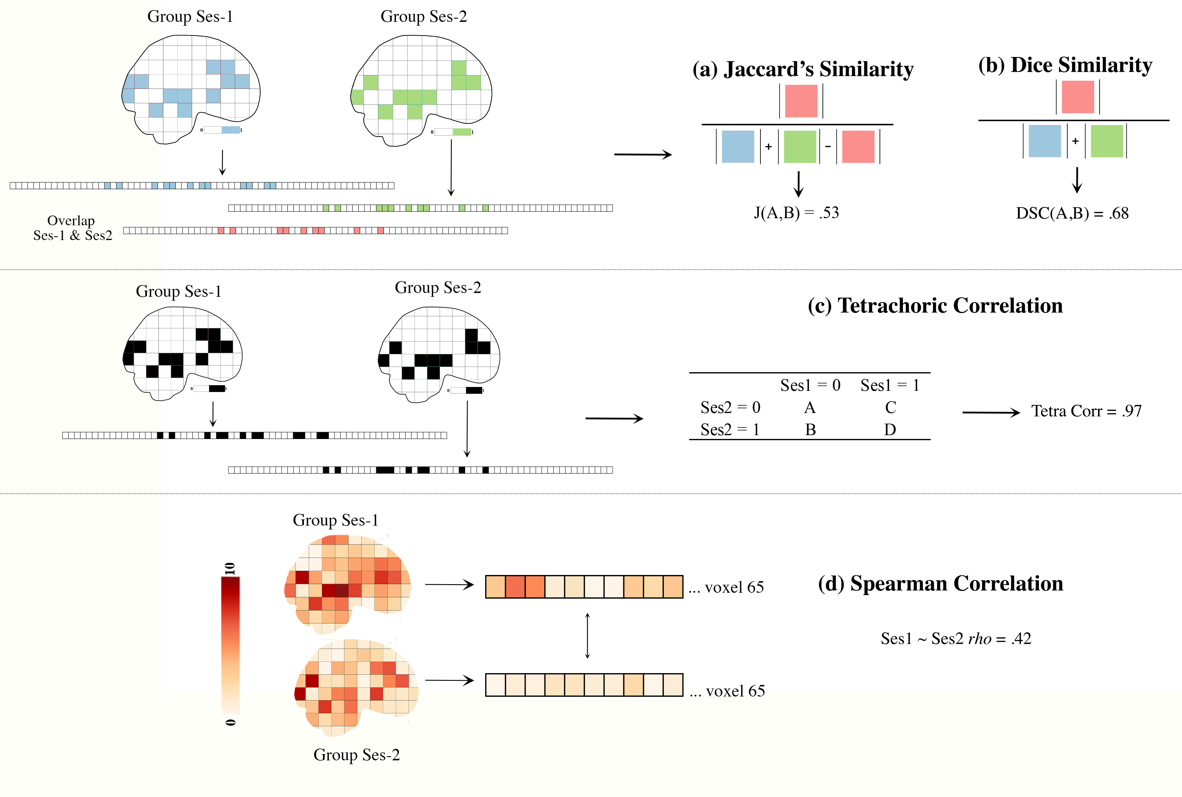
Figure 3. Similarity Between Images
tetrachoric_correlation
From pyrelimri, the tetrachoric_correlation module contains functions to calculate tetrachoric correlation between binary images.
tetrachoric_corr
- pyrelimri.tetrachoric_correlation.tetrachoric_corr(vec1: ndarray, vec2: ndarray) float[source]
Calculates the tetrachoric correlation between two binary vectors, vec1 and vec2.
- Parameters:
vec1 – A 1D binary numpy array of length n representing the 1st dichotomous (1/0) variable.
vec2 – A 1D binary numpy array of length n representing the 2nd dichotomous (1/0) variable..
Returns: The tetrachoric correlation between the two binary variables.
conn_icc
The conn_icc module is a wrapper for the icc module, specifically focusing on edge-wise intraclass correlation coefficient calculations.
edgewise_icc
- pyrelimri.conn_icc.edgewise_icc(multisession_list: list, n_cols: int, col_names: list = None, separator=None, icc_type='icc_3')[source]
Calculates the Intraclass Correlation Coefficient (ICC), its confidence intervals (lower and upper bounds) and between subject, within subject and between measure variance components for each edge within specified input files or NDarrays using manual sum of squares calculations. The path to the subject’s data (or ndarrays) should be provided as a list of lists for each session.
Example of input lists for three sessions: dat_ses1 = [“./ses1/sub-01_ses-01_task-pilot_conn.csv”, “./ses1/sub-02_ses-01_task-pilot_conn.csv”, “./ses1/sub-03_ses-01_task-pilot_conn.csv”] dat_ses2 = [“./ses2/sub-01_ses-02_task-pilot_conn.csv”, “./ses2/sub-02_ses-02_task-pilot_conn.csv”, “./ses2/sub-03_ses-02_task-pilot_conn.csv”] dat_ses3 = [“./ses3/sub-01_ses-03_task-pilot_conn.csv”, “./ses3/sub-02_ses-03_task-pilot_conn.csv”, “./ses3/sub-03_ses-03_task-pilot_conn.csv”]
The order of the subjects in each list must be the same.
Two session example: multisession_list = [dat_ses1, dat_ses2] Three session example: multisession_list = [dat_ses1, dat_ses2, dat_ses3]
Inter-subject variance: between subjects in sessions 1, 2, and 3 Intra-subject variance: within subject across sessions 1, 2, and 3
- Parameters:
multisession_list (list of lists) – Contains paths to .npy files or NDarrays for subjects’ connectivity MxN square matrices for each session.
n_cols (int) – Expected number of columns/rows in the NxN matrix.
col_names (list of str, optional) – List of column names corresponding to the MxN matrix. Defaults to None.
separator (str, optional) – If multisession_list contains file paths and not .npy extension, provide separator to load dataframes, e.g., ‘,’ or ‘ ‘. Defaults to None.
icc_type (str, optional) – Specify ICC type. Default is ‘icc_3’. Options: ‘icc_1’, ‘icc_2’, ‘icc_3’.
- Returns:
- A dictionary with the following keys:
’roi_labels’: List of column names representing the connectivity edges.
’est’: Estimated ICCs as a 2D matrix.
’lowbound’: Lower bounds of ICC confidence intervals as a 2D matrix.
’upbound’: Upper bounds of ICC confidence intervals as a 2D matrix.
’btwn_sub’: Between-subject variance as a 2D matrix.
’wthn_sub’: Within-subject variance as a 2D matrix.
’btwn_meas’: Between-measure variance as a 2D matrix.
- Return type:
dict
Example
- icc_results = edgewise_icc(multisession_list=[dat_ses1, dat_ses2, dat_ses3],
n_cols=10, col_names=[‘left_pfc’, ‘right_pfc’, …, ‘right_nacc’], separator=’,’, icc_type=’icc_3’)
masked_timeseries
The masked_timeseries module extracts timeseries data from BOLD images for regions of interest (ROI).
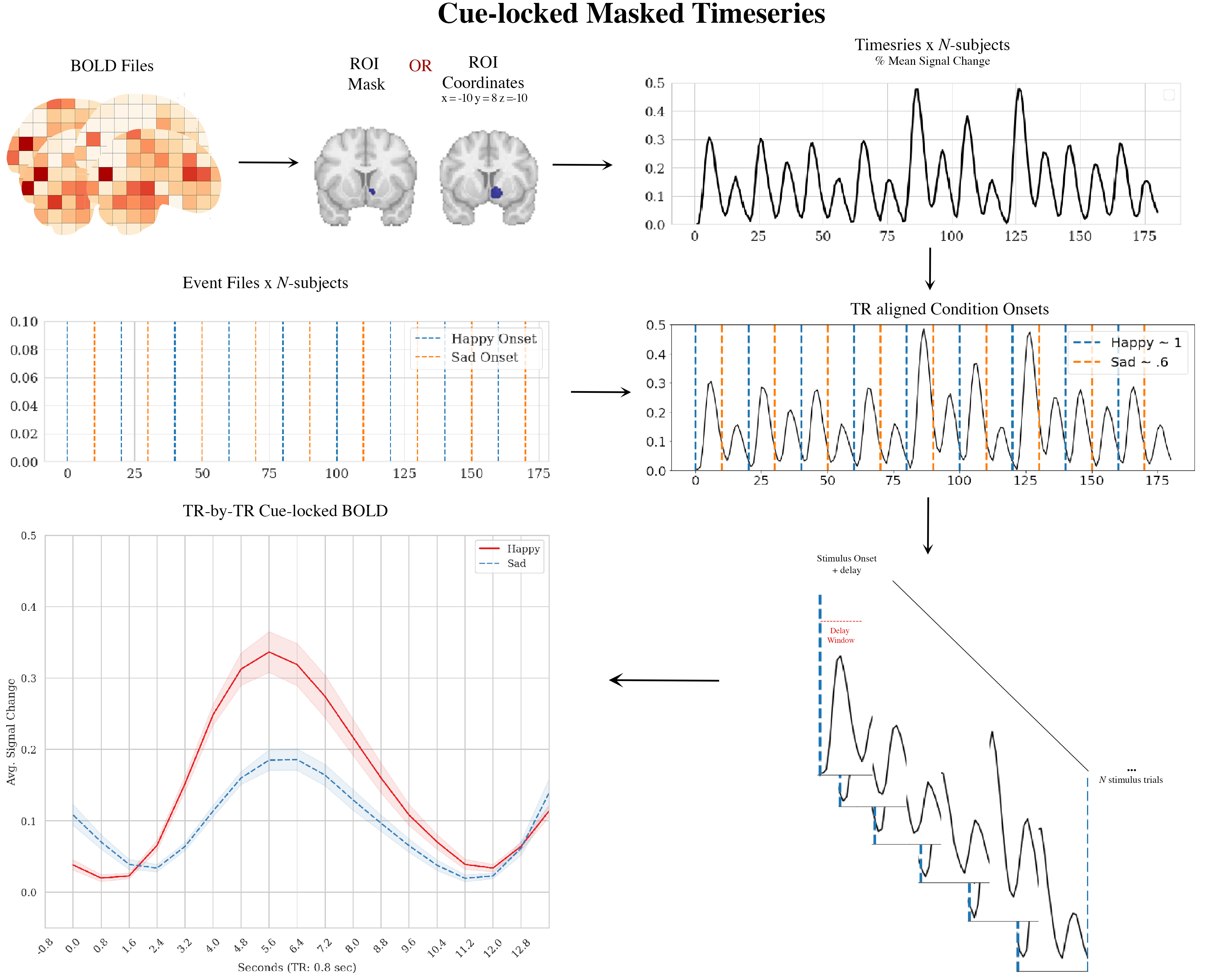
Figure 4. Masked Timeseries Illustration
extract_time_series
- pyrelimri.masked_timeseries.extract_time_series(bold_paths: list, roi_type: str, high_pass_sec: int = None, roi_mask: str = None, roi_coords: tuple = None, radius_mm: int = None, detrend: bool = False, fwhm_smooth: float = None, n_jobs=1)[source]
Extracts time series data from BOLD images for specified regions of interest (ROI) or coordinates. For each BOLD path, extracts time series either using a mask or ROI coordinates, leveraging Nilearn’s NiftiLabelsMasker (for mask) or nifti_spheres_masker (for coordinates). BOLD signal using Nilearn’s percent signal change (‘psc’)
- Parameters:
bold_paths (list) – List of paths to BOLD image files for subjects/runs/tasks. The order should match the order of events or conditions for each subject.
roi_type (str) – Type of ROI (‘mask’ or ‘coords’).
high_pass_sec (int, optional) – High-pass filter cutoff in seconds. If provided, converted to frequency (1/high_pass_sec). Default is None.
roi_mask (str or None, optional) – Path to the ROI mask image. Required if roi_type is ‘mask’. Default is None.
roi_coords (tuple or None, optional) – Coordinates (x, y, z) for the center of the sphere ROI. Required if roi_type is ‘coords’. Default is None.
radius_mm (int or None, optional) – Radius of the sphere in millimeters. Required if roi_type is ‘coords’. Default is None.
detrend (bool, optional) – Whether to detrend the BOLD signal using Nilearn’s detrend function. Default is False.
fwhm_smooth (float or None, optional) – Full-width at half-maximum (FWHM) value for Gaussian smoothing of the BOLD data. Default is None.
n_jobs (int, optional) – Number of CPUs to use for parallel processing. Default is 1.
- Returns:
- If roi_type is ‘mask’:
List of numpy arrays containing the time series (% mean signal change) data for each subject/run.
List of subject information strings formatted as ‘sub-{sub_id}_run-{run_id}’.
- If roi_type is ‘coords’:
List of numpy arrays containing the averaged time series (% mean signal change) data for each subject/run.
Nifti1Image object representing the coordinate mask used.
List of subject information strings formatted as ‘sub-{sub_id}_run-{run_id}’.
- Return type:
list or tuple
Example
# Extract percent mean signal change time series for BOLD data using a mask ROI roi_type = ‘mask’ bold_paths = [‘./sub-01_ses-01_task-lit_bold.nii.gz’, ‘./sub-02_ses-01_task-lit_bold.nii.gz’] roi_mask = ‘./siq-roi_mask.nii.gz’ time_series_list, sub_info_list = extract_time_series(bold_paths, roi_type, roi_mask=roi_mask, high_pass_sec=100, detrend=True, fwhm_smooth=5.0)
# Extract percent mean signal change time series for BOLD data using coordinates ROI roi_type = ‘coords’ bold_paths = [‘./sub-01_ses-01_task-lit_bold.nii.gz’, ‘./sub-02_ses_1_task-lit_bold.nii.gz’] roi_coords = (30, -15, 0) time_series_list, coord_mask, sub_info_list = extract_time_series(bold_paths, roi_type, roi_coords=roi_coords, radius_mm=5, high_pass_sec=100, detrend=True, fwhm_smooth=5.0)
extract_postcue_trs_for_conditions
- pyrelimri.masked_timeseries.extract_postcue_trs_for_conditions(events_data: list, onset: str, trial_name: str, bold_tr: float, bold_vols: int, time_series: ndarray, conditions: list, tr_delay: int, list_trpaths: list)[source]
Extracts time points coinciding with condition onsets plus specified delay TRs for each subjects’ behavioral/timeseries data. Saves this information to a pandas DataFrame with associated mean signal values for each subject, trial and cue across the range of TRs (1 to TR-delay).
- Parameters:
events_data (list) – List of paths to behavioral data files. Should match the order of subjects/runs/tasks as the BOLD file list.
onset (str) – Name of the column containing onset values in the behavioral data.
trial_name (str) – Name of the column containing condition values in the behavioral data.
bold_tr (float) – TR (Repetition Time) for acquisition of BOLD data in seconds.
bold_vols (int) – Number of volumes for BOLD acquisition.
time_series (numpy.ndarray) – series_list from extract_time_series()
conditions (list) – List of condition cues to iterate over. Must have at least one cue.
tr_delay (int) – Number of TRs after onset of stimulus to extract and plot.
list_trpaths (list) – id_list from extract_time_series()
- Returns:
DataFrame containing percent mean signal change values, subject labels, trial labels, TR values, and cue labels for all specified conditions.
- Return type:
pd.DataFrame
Example
# Extract time points and mean signal values for conditions ‘A’ and ‘B’ events_dfs = [‘./sub-01_ses-01_task-siq-events.csv’, ‘./sub-02_ses-01_task-siq-events.csv’] onset = ‘OnsetTime’ trial_name = ‘TrialType’ timeseries_2subs = series list from extract_time_series() conditions = [‘Up’, ‘Down’] tr_delay = 5 timeseries_order = id_list from extract_time_series() result_df = extract_postcue_trs_for_conditions(events_data=events_dfs, onset=’OnsetTime’, trial_name=’TrialType’, bold_tr=2.0, bold_vols=150, time_series=timeseries_2subs, conditons=[‘Up’,’Down’], tr_delay=12, list_trpaths=timeseries_order)
plot_responses
- pyrelimri.masked_timeseries.plot_responses(df, tr: int, delay: int, style: str = 'white', save_path: str = None, show_plot: bool = False, ylim: tuple = (-1, 1))[source]
Plots the BOLD response (Mean_Signal ~ TR) across the specified delay for cues. The plot uses an alpha of 0.1 with n = 1000 bootstraps for standard errors.
- Parameters:
df (pandas.DataFrame) – DataFrame containing the data to plot from extract_postcue_trs_for_conditions(). Should include columns ‘TR’, ‘Mean_Signal’, and ‘Cue’.
tr (int) – TR value in seconds.
delay (int) – Delay value indicating the number of TRs to plot.
style (str, optional) – Style of the plot. Options are ‘white’ or ‘whitegrid’. Default is ‘white’.
save_path (str, optional) – Path and filename to save the plot. If None, the plot is not saved. Default is None.
show_plot (bool, optional) – Whether to display the plot. Default is False.
ylim (tuple, optional) – Y-axis limits for the plot. Default is (-1, 1).
- Return type:
If show_plot = True, open backend graphics to view figure