Intraclass Correlation Functions
The intraclass correlation (ICC) estimates are a complement to the similarity functions. The variability/similarity in the data can be parsed in several ways. One can estimate how similar things are above a threshold (e.g., 1/0) or how similar specific continuous estimates are across subjects. The ICC is used for the latter.
Two modules with examples are reviewed here: The icc, brain_icc and conn_icc modules. The first is the manual estimation of the ICC estimates, such as the (1) \(SS_{total}\), the (2) \(SS_{within}\), (3) \(SS_{Between}\) their associated mean sums of squares (which is a decomposition of variance 1-3 divided by specific degrees of freedoms) in the icc module. Then, these ICC estimates are calculated on a voxel-by-voxel basis (or if you wanted to, ROI by ROI) using brain module. and roi-by-roi basis using ‘roi_icc’. Finally, an example is provided using the conn_icc module to estimate edgewise ICC on matrices.
icc
While icc is within the package for MRI reliability estimates, it can still be used to calculate different values on dataframes. Below I describe the different components and use seaborns.anagrams as the example for each of these components.
The first 5-rows of the anagrams data are:
subidr |
attnr |
num1 |
num2 |
num3 |
|---|---|---|---|---|
1 |
divided |
2 |
4 |
7 |
2 |
divided |
3 |
4 |
5 |
3 |
divided |
3 |
5 |
6 |
4 |
divided |
5 |
7 |
5 |
5 |
divided |
4 |
5 |
8 |
We can load the example data, filter to only use the divided values and convert the data into a long data format:
import seaborn as sns
data = sns.load_dataset('anagrams') # load
a_wd = data[data['attnr'] == 'divided'] # filter
# convert to wide, so the subject/id variables are still `subidr` and values were stacking from `num1`,`num2`,num3`
# the values will be stored in the column `vals` and the session labels (from num1-num3) into `sess`
long_df = pd.DataFrame(
    pd.melt(a_wd,
           id_vars="subidr",
           value_vars=["num1", "num2", "num3"],
           var_name="sess",
           value_name="vals"))
sumsq_total
The sum of squared total is the estimate of the total variance across all subjects and measurement occasions. Expressed by formula:
- where:
\(df_{long}\) = pandas DataFrame (df) in long format
values = is a variable string for the values containing the scores in df
\(x_i\) = is each value in the column specified by values column in df
\(\bar x\) = is the global mean specified by ‘values’ column in df
Using the anagrams long_df I’ll calculate the sum of square total using:
from pyrelimri import icc
icc.sumsq_total(df_long=long_df, values="vals")
We will get the result of 71.8 sum of squared total.
sumsq_within
- where:
\(df_{long}\) = pandas DataFrame in long format
sessions = is a session (repeated measurement) variable, string, in df
values = is a variable, string, for the values containing the scores in df
\(n_{subjects}\) = the number of subjects in df
\(\bar x_i\) = is the mean of the values column for session i in df
\(\bar x\) = is the global mean specified by ‘values’ column in df
m = is the number of sessions
We can calculate the sum of squares within using the below:
# if you havent imported the package already
from pyrelimri import icc
icc.sumsq_within(df_long=long_df, sessions="sess", values="vals", n_subjects=10)
We will get the result of 29.2 sum of squares between subject factor.
sumsq_btwn
- where:
\(df_{long}\) = pandas DataFrame in long format
subj = is the subject variable, string, in df
values = is a variable, string, for the values containing the scores in df
\(n_{sessions}\) = the number of sessions in df
\(\bar x_i\) = is the mean of the values column for subject i in df
\(\bar x\) = is the global mean specified by ‘values’ column in df
s = is the number of subjects
# if you havent imported the package already
from pyrelimri import icc
icc.sumsq_btwn(df_long=long_df, subj="subidr", values="vals", n_sessions=3) # 3 = num1-num3
We will get the result of 20.0 sum of squares between subject factor.
Note: If you recall that ICC is the decomposition of total variance, you’ll notice that 29.2 + 20.0 do not sum to the total variance, 71.8. This is because there is the subj*sess variance component and the residual variance, too. You can review this in an ANOVA table:
# if you havent imported the package already
from pinguin import anova
round(anova(dv='vals', between=['subidr','sess'], data=long_df, detailed=True),3)
icc_confint
For each ICC estimate that can be requested, ICC(1), ICC(2,1) and ICC(3,1), a confidence interval is returned for each associated ICC estimate. The implementation for the confidence interval is the same as in the the pingouin package in Python and the ICC() from psych package in R.
sumsq_icc
Now that the internal calculations of the ICC have been reviewed, I will use the package to get the values of interest. The formulas for the ICC(1), ICC(2,1) and ICC(3,1) are described below.
Where:
\(BS_{Btwn}\): mean square between subjects
\(MS_{Wthn}\): mean square within subjects
\(MS_{Err}\): mean squared residual error
\(MS_{Sess}\): mean squared error of sessions
\(\bar x\): is the number of sessions
\(N_{subjs}\): numbers of subjects
In terms to the above ICC(1), ICC(2,1) and ICC(3,1) formulas, these are also written in Table 1 in Liljequist et al., 2019 as below. These are in terms of between subject variance (deviation from mean for \(subject_i\) = \(\sigma_r^2\)), noise/within subject variance (variance in measurement \(j\) for \(subject_i\) = \(\sigma_v^2\)), and measurement additive bias (bias in measurement \(j\) = \(\sigma_c^2\)):
Hence, sumsq_icc can be used on a dataset with multiple subjects with 1+ measurement occasions. The ICC can be calculated for the anagrams data references above. Note: the required inputs are a long dataframe, subject variable, session variable and the value scores variables that are contained in the long dataframe, plus the icc to return (options: icc_1, icc_2, icc_3; default: icc_3).
The sumsq_icc function will return [six] values: the ICC estimate, lower bound 95% confidence interval, upper bound 95% confidence interval and specific to each computation, the between-subject variance (\(\sigma_r^2\)), within subject variance (\(\sigma_v^2\)), and in case of ICC(2,1) between-measure variance (\(\sigma_c^2\)). This information will print to the terminal or can be saved to six variables. Example:
# if you havent imported the package already
from pyrelimri import icc

icc3, icc3_lb, icc3_up, icc3_btwnsub, \
icc3_withinsub, _ = icc.sumsq_icc(df_long=a_ld,sub_var="subidr",
                                          sess_var="sess",value_var="vals",icc_type="icc_3")
- This will store the five associated values in the five variables:
icc3: ICC estimate
icc3_lb: 95% lower bound CI for ICC estimate
icc3_lb: 95% upper bound CI for ICC estimate
icc3_btwnsub: Between Subject Variance used for ICC estimate (\(\sigma_r^r\))
icc3_withinsub: Within Subject Variance used for ICC estimate (\(\sigma_r^v\))
icc3_btwnmeas: setting to _ as between measure variance is not computed for ICC(3,1) (\(\sigma_c^2\))
Reminder: If NaN/missing values, icc implements a mean replacement of all column values. If this is not preferred, handle missing/unbalanced cases beforehand.
brain_icc
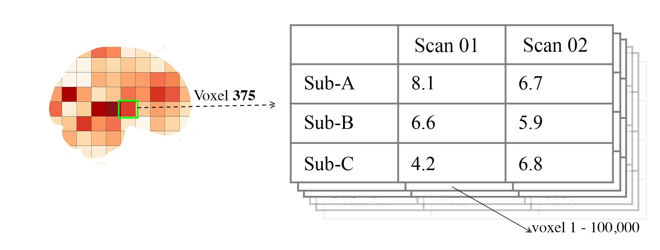
The brain_icc module is a big wrapper for for the icc module. In short, the voxelwise_icc function within the brain_icc modules calculates the ICC for 3D nifti brain images across subjects and sessions on a voxel-by-voxel basis.
Here are the steps it uses:
Function takes a list of paths to the 3D nifti brain images for each session, the path to the nifti mask object, and the ICC type to be calculated.
Function checks if there are the same number of files in each session (e.g., list[0], list[1], etc) and raises an error if they are of different length.
Function concatenates the 3D images into a 4D nifti image (4th dimension is subjects) using image.concat_imgs().
Function uses the provided nifti mask to mask the images using NiftiMasker.
Function loops over the voxels in the imgdata[0].shape[-1] and creates a pandas DataFrame with the voxel values for each subject and session using sumsq_icc().
The function calculates and returns a dictionary with five 3D volumes: est, lower (lower_bound) and upper (upper_bound) of the ICC 95% confidence interval, and between subject, within subject and between measure variance from sumsq_icc().
Note, the shape of the provided 3D volume is determined using inverse_transform from NiftiMasker.
voxelwise_icc
As mentioned above, the voxelwise_icc calculates the ICC values for each voxel in the 3D volumes. Think of an image as having the dimensions of [45, 45, 90], that can be unraveled to fit into a single vector for each subject that is 182,250 values long (the length in the voxelwise case is the number of voxels). The voxelwise_icc returns an equal size in length array that contains the ICC estimate for each voxels, between subjects across the measurement occasions. For example:
- To use the voxelwise_icc function, you have to provide the following information:
multisession_list: A list of listed paths to the Nifti z-stat, t-stat or beta maps for sess1, 2, 3, etc (or run 1,2,3..)
mask: The Nifti binarized masks that will be used to mask the 3D volumes.
icc_type: The ICC estimate that will be calculated for each voxel. Options: icc_1, icc_2, icc_3. Default: icc_3
- The function returns a dictionary with 3D volumes for:
ICC estimates (‘est’)
ICC lowerbound 95% CI (‘lowbound’)
ICC upperbound 95% CI (‘upbound’)
Between Subject Variance (‘btwnsub’)
Within Subject Variance (‘wthnsub’)
Between Measure Variance (‘btwnmeas’)
So the resulting stored variable will be a dictionary, e.g. “brain_output”, from which you can access to view and save images such as the ICC estimates (brain_output[‘est’]) and/or within subject variance (brain_output[‘wthnsub’]).
Say I have stored paths to session 1 and session 2 in the following variables (Note: subjects in list have same order!):
# session 1 paths
scan1 = ["./scan1/sub-1_t-stat.nii.gz", "./scan1/sub-2_t-stat.nii.gz", "./scan1/sub-3_t-stat.nii.gz", "./scan1/sub-4_t-stat.nii.gz", "./scan1/sub-5_t-stat.nii.gz",
         "./scan1/sub-6_t-stat.nii.gz", "./scan1/sub-7_t-stat.nii.gz", "./scan1/sub-8_t-stat.nii.gz"]
scan2 = ["./scan2/sub-1_t-stat.nii.gz", "./scan2/sub-2_t-stat.nii.gz", "./scan2/sub-3_t-stat.nii.gz", "./scan2/sub-4_t-stat.nii.gz", "./scan2/sub-5_t-stat.nii.gz",
         "./scan2/sub-6_t-stat.nii.gz", "./scan2/sub-7_t-stat.nii.gz", "./scan2/sub-8_t-stat.nii.gz"]
Next, I can call these images paths in the function and save the 3d volumes using (running 4 processes in parallel with n_jobs = 4):
from pyrelimri import brain_icc

brain_icc_dict = brain_icc.voxelwise_icc(multisession_list = [scan1, scan2], mask = "./mask/brain_mask.nii.gz", icc_type = "icc_3", n_jobs = 4)
This will return the associated dictionary with nifti 3D volumes which can be manipulated further.
Here I plot the icc estimates (i.e. ‘est’) using nilearn’s plotting
from nilearn.plotting import view_img_on_surf

view_img_on_surf(stat_map_img = brain_icc_dict["est"],
                 surf_mesh = 'fsaverage5', threshold = 0,
                 title_fontsize = 16, colorbar_height = .75,
                 colorbar_fontsize = 14).open_in_browser()
Here I save the image using nibabel:
import nibabel as nib
    nib.save(brain_icc_dict["est"], os.path.join('output_dir', 'file_name.nii.gz'))
Here is a real-world example using neurovaults data collection for Precision Functional Mapping of Individual brains. The collection is: 2447. The neurovault collection provides data for ten subjects, with ten sessions. I will use the first two sessions. I will use the block-design motor task and focus on the [Left] Hand univariate beta maps which are listed under “other”.
Let’s use nilearn to load these data for 10 subjects and 2 sessions.
from nilearn.datasets import fetch_neurovault_ids
# Fetch left hand motor IDs
MSC01_ses1 = fetch_neurovault_ids(image_ids=[48068]) # MSC01 motor session1 1 L Hand beta
MSC01_ses2 = fetch_neurovault_ids(image_ids=[48073]) # MSC01 motor session2 1 L Hand beta
MSC02_ses1 = fetch_neurovault_ids(image_ids=[48118])
MSC02_ses2 = fetch_neurovault_ids(image_ids=[48123])
MSC03_ses1 = fetch_neurovault_ids(image_ids=[48168])
MSC03_ses2 = fetch_neurovault_ids(image_ids=[48173])
MSC04_ses1 = fetch_neurovault_ids(image_ids=[48218])
MSC04_ses2 = fetch_neurovault_ids(image_ids=[48223])
MSC05_ses1 = fetch_neurovault_ids(image_ids=[48268])
MSC05_ses2 = fetch_neurovault_ids(image_ids=[48273])
MSC06_ses1 = fetch_neurovault_ids(image_ids=[48318])
MSC06_ses2 = fetch_neurovault_ids(image_ids=[48323])
MSC07_ses1 = fetch_neurovault_ids(image_ids=[48368])
MSC07_ses2 = fetch_neurovault_ids(image_ids=[48368])
MSC08_ses1 = fetch_neurovault_ids(image_ids=[48418])
MSC08_ses2 = fetch_neurovault_ids(image_ids=[48423])
MSC09_ses1 = fetch_neurovault_ids(image_ids=[48468])
MSC09_ses2 = fetch_neurovault_ids(image_ids=[48473])
MSC10_ses1 = fetch_neurovault_ids(image_ids=[48518])
MSC10_ses2 = fetch_neurovault_ids(image_ids=[48523])
Now that the data are loaded, I specify the session paths (recall, Nilearn saves the paths to the images on your computer) and then I will provide this information to voxelwise_icc function within brain_icc module
# session 1 list from MSC
sess1_paths = [MSC01_ses1.images[0], MSC02_ses1.images[0], MSC03_ses1.images[0],
               MSC04_ses1.images[0], MSC05_ses1.images[0], MSC06_ses1.images[0],
               MSC07_ses1.images[0], MSC08_ses1.images[0],MSC09_ses1.images[0],
               MSC10_ses1.images[0]]
# session 2 list form MSC
sess2_paths = [MSC01_ses2.images[0], MSC02_ses2.images[0], MSC03_ses2.images[0],
               MSC04_ses2.images[0], MSC05_ses2.images[0], MSC06_ses2.images[0],
               MSC07_ses2.images[0], MSC08_ses2.images[0],MSC09_ses2.images[0],
               MSC10_ses2.images[0]]
Notice, the function asks for a mask. These data do not have a mask provided on neurovault, so I will calculate one on my own and save it to the filepath of these data using nilearns multi-image masking option.
from nilearn.masking import compute_multi_brain_mask
import nibabel as nib
import os # so Ican use only the directory location of the MSC img path

mask = compute_multi_brain_mask(target_imgs = sess1_paths)
mask_path = os.path.join(os.path.dirname(MSC01_ses1.images[0]), 'mask.nii.gz')
nib.save(mask, mask_path)
Okay, now I have everything I need: the paths to the images and to the mask.
from pyrelimri import brain_icc

brain_icc_msc = brain_icc.voxelwise_icc(multisession_list = [sess1_paths, sess2_paths ],
                                        mask=mask_path, icc_type='icc_1', n_jobs = 4)
Since the dictionary is saved within the environment, you should see the dictionary with five items. On my mac (i9, 16GM mem), it took ~4minutes to run this and get the results. Time will depend on the size of data and your machine.
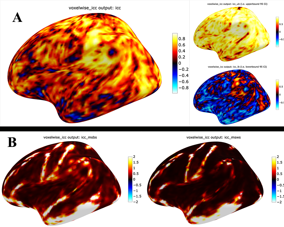
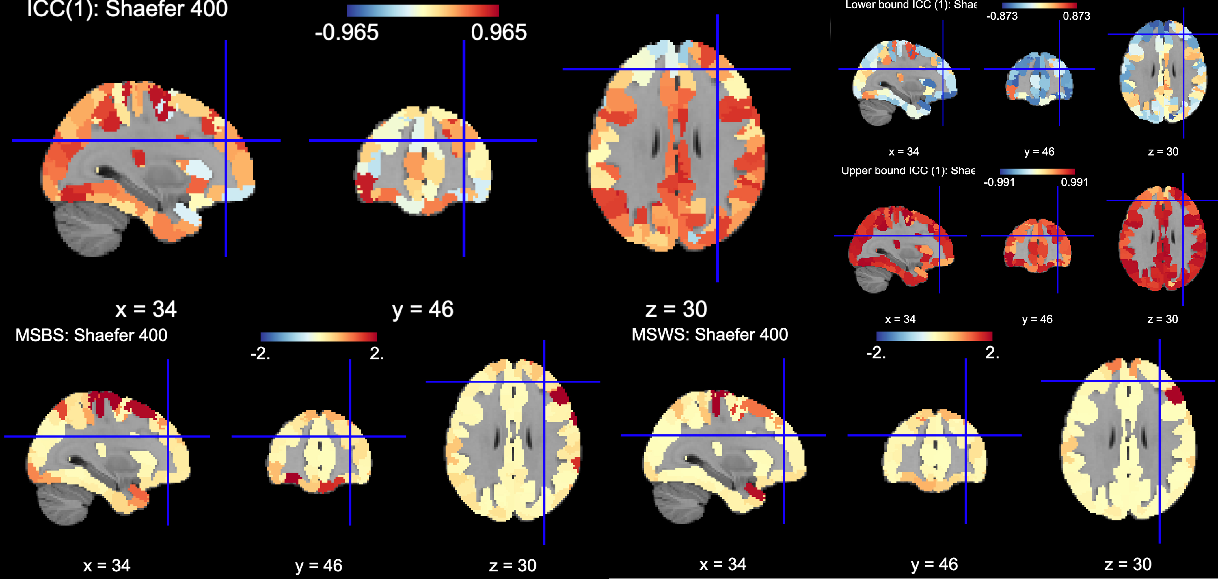
You can plot the volumes using your favorite plotting method in Python. For this example. Figure 2A shows the three 3D volumes for ICC, 95% upper bound and 95% lower bound. Then, Figure 2B shows the two different variance components, mean squared between subject (msbs) and mean squared within subject (msws) variance. Note, depending on the map will determine the thresholding you may want to use. Some voxels will have quite high variability so here the example is thresholded +2/-2. Alternatively, you can standardize the values within the image before plotting to avoid issues with outliers.
As before, you can save out the images using nibabel to a directory. Here I will save it to where the images are stored:
import nibabel as nib
nib.save(brain_icc_msc["est"], os.path.join('output_dir', 'MSC-LHandbeta_estimate-icc.nii.gz'))
nib.save(brain_icc_msc["btwnsub"], os.path.join('output_dir', 'MSC-LHandbeta_estimate-iccbtwnsub.nii.gz'))
roi_icc
Similar to the steps described for voxelwise_icc above, the brain_icc module includes the option to calculate ICC values based on a pre-specified probablistic or determistic Nilearn Atlas. As mentioned elsewhere, the atlases are described on Nilearn datasets webpage.
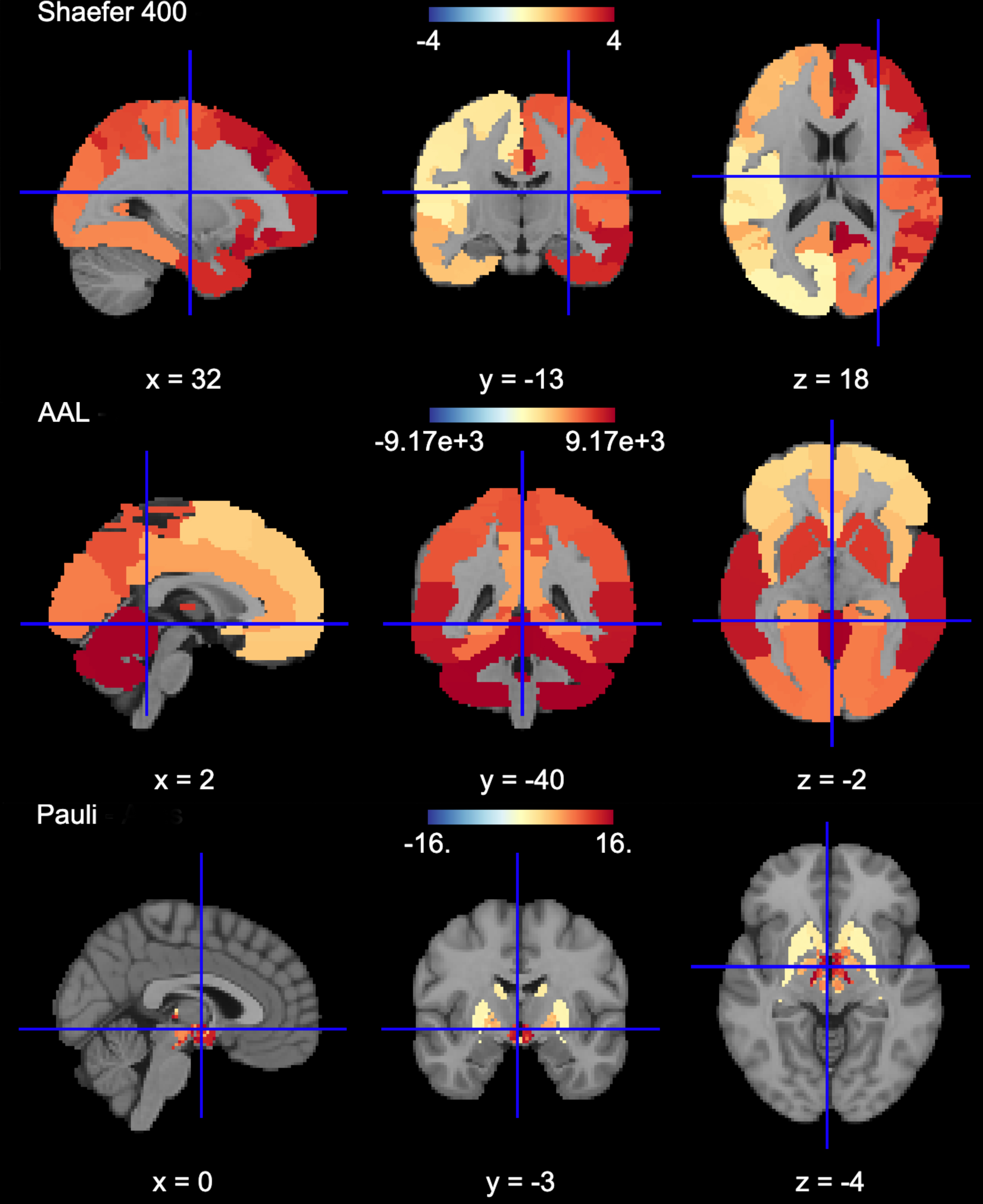
The Determistic atlas options (visual ex. Figure 3):
AAL, Destrieux 2009, Harvard-Oxford, Juelich, Pauli 2017, Shaefer 2018, Talairach
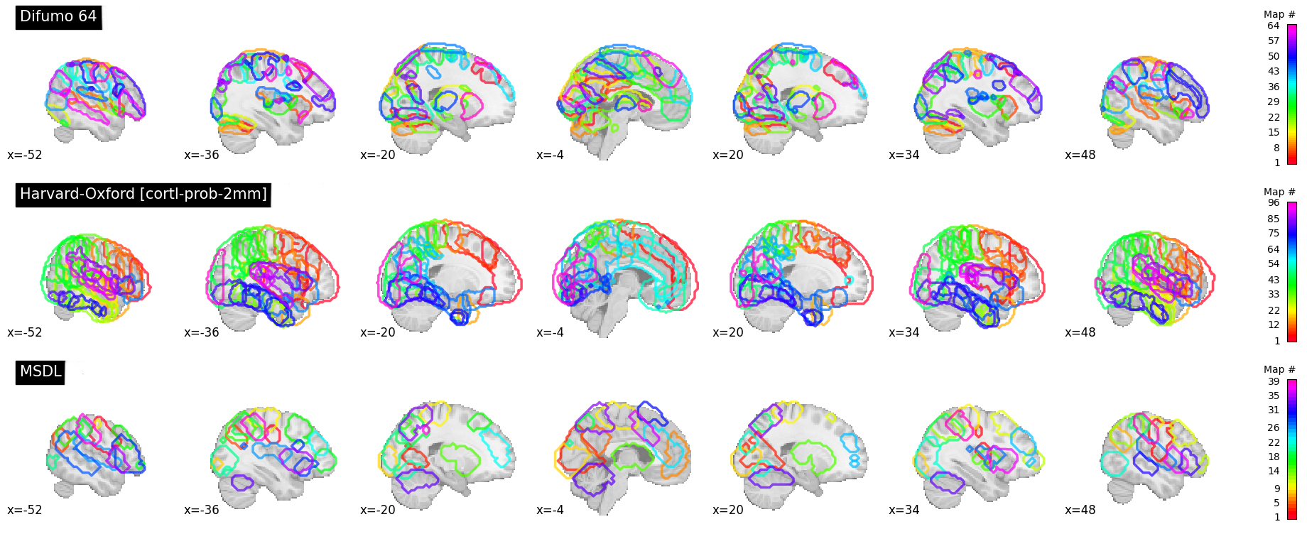
The Probabilistic atlas options (visual ex. Figure 4):
Difumo, Harvard-Oxford, Juelich and Pauli 2017
Using the same MSC Neurovault data from above, the method to calculate ROI based ICCs is nearly identical to voxelwise_icc() with a few exceptions. First, since I am masking the data by ROIs (e.g., atlas), a mask is not necessary. Second, since the atlas and data may be in different affine space, to preserve the boundaries of ROIs the deterministic atlases as resampled to the atlas (e.g., NiftiLabelsMasker(… resampling_target = ‘labels’)). However, as the boundaries are less clear for probabilistic atlases and the compute time is decreased, the atlas is resampled to the data (e.g. in NiftiMapssMasker(… resampling_target = ‘data’). Third, the resulting dictionary will contain 11 variables:
Atlas ROI Labels (‘roi_labels’): This contains the order of labels (e.g., pulled from atlas.labels)
ICC estimates (‘est’): 1D array that contains ICCs estimated for N ROIs in atlas (atlas.maps[1:] to skip background).
ICC lower bound (lb) 95% CI (‘lowbound’): 1D array that contains lb ICCs estimated for N ROIs in atlas.
ICC upper bound (up) 95% CI (‘upbound’): 1D array that contains ub ICCs estimated for N ROIs in atlas.
Between Subject Variance (‘btwnsub’): 1D array that contains between subject variance estimated for N ROIs in atlas.
Within Subject Variance (‘wthnsub’): 1D array that contains within subject variance estimated for N ROIs in atlas.
Between Measure Variance (‘btwnmeas’): 1D array that contains between measure variance estimated for N ROIs in atlas (ICC[2,1] only, otherwise filled None)
ICC estimates transformed back to space of ROI mask (‘est_3d’): Nifti 3D volume of ICC estimates
ICC lower bound 95% CI transformed back to space of ROI mask (‘lowbound_3d’): Nifti 3D volume of lb ICC estimates
ICC upper bound 95% CI transformed back to space of ROI mask (‘upbound_3d’): Nifti 3D volume of up ICC estimates
Between Subject Variance transformed back to space of ROI mask (‘btwnsub_3d’): Nifti 3D volume of between subject variance estimates
Within Subject Variance transformed back to space of ROI mask (‘wthnsub_3d’): Nifti 3D volume of within subject variance estimates
Between Measure Variance transformed back to space of ROI mask (‘btwnmeas_3d’): Nifti 3D volume of between measure variance estimates
An important caveat: Probabilistic atlases are 4D volumes for N ROIs. This is because each voxel has an associated probability that it belongs to ROI A and ROI B. Thus, ROIs may overlap and so the estimates (as in example below) will be more smooth.
Here is an example to run roi_icc using the MSC data loaded above for the deterministic Shaefer 400 ROIs atlas. We call the roi_icc function within the brain_icc module, specify the multisession list of data, the atlas, defaults and/or requirements the atlas requires (e.g., here, I specify n_rois = 400 which is the default), the directory where I want to save the atlas (I chose ‘/tmp/’ on Mac) and the icc type (similar as above, ICC[1])
from pyrelimri import brain_icc

shaefer_icc_msc = brain_icc.roi_icc(multisession_list=[sess1_paths,sess2_paths],
                                type_atlas='shaefer_2018', n_rois = 400,
                                atlas_dir='/tmp/', icc_type='icc_1')
This will run A LOT faster than the voxelwise_icc method as ‘roi_icc’ is reducing the voxel dimensions to ROI dimension (slower for probabilistic) and looping over the length of ROIs in the atlas. So in many cases it is reducing 200,000 voxel calculations to 400 ROI calculations.
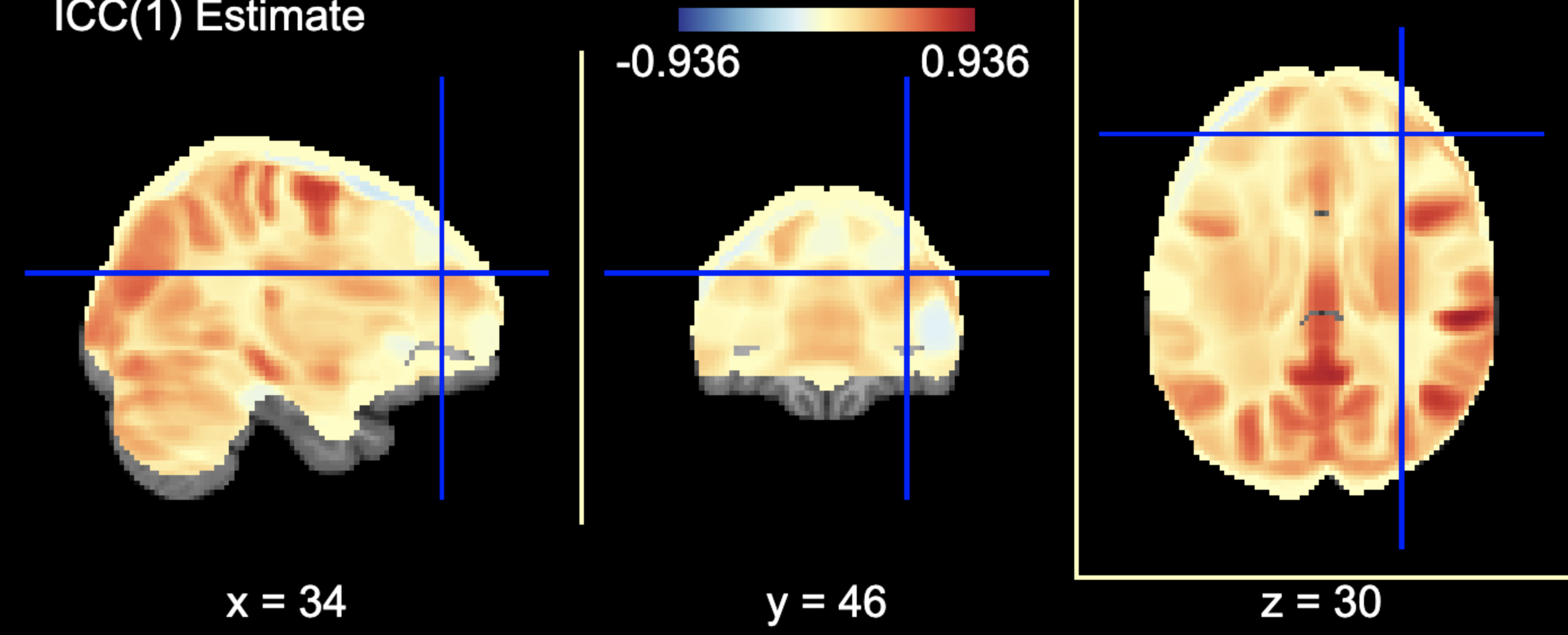
You can access the array of estimates and plot the Nifti image using: .. code-block:: python
from nilearn import plotting
# access estimates for ICC values shaefer_icc_msc[‘est’]
# plot estimate nifti volume plotting.plot_stat_map(stat_map_img=shaefer_icc_msc[‘est_3d’], title=’ICC(1) Estimate’)
Figure 5 is a visual example of est_3d, lowerbound_3d, upperbound_3d, btwnsub_3d, wthnsub_3d, ‘btwnmeas_3d’ for the 400 ROI Shaefer atlas.
I can do the same for a probabilistic atlas – say the 256 ROI Difumo atlas.
from pyrelimri import brain_icc

difumo_icc_msc = brain_icc.roi_icc(multisession_list=[sess1_paths,sess2_paths],
                                type_atlas='difumo', dimension = 256, # notice, 'dimension' is unqiue to this atlas
                                atlas_dir='/tmp/', icc_type='icc_1')
Figure 6 contains the estimates from the Difumo 256 atlas. Again, since this is a probabilistic atlas each voxel has an association probability belonging to each ROI and so there are not clear boundaries. The data will have slightly different distributions and appear more smooth so interpreting the maps should be approached with this in mind.
conn_icc
The conn_icc module is a wrapper for for the icc module. In short, the edgewise_icc function, like voxelwise_icc within the brain_icc module, calculates the ICC for an NxN matrix across subjects and sessions on a cell-by-cell basis (or edge-by-edge).
Here are the steps it uses:
Function takes list of subject a) paths to .npy, .txt, .csv correlation matrices or b) numpy arrays for each session, the number of columns in each matrix (e.g., ROI names), the list of column names (if not provided, populates as 1:len(number columes) and the ICC type to be calculated.
Function checks the list names and number of columns match and confirms N per session is the same.
If the list of lists are strings, the files are loaded based on .npy, .txt or .csv extensive with provided separator. If .csv pandas assumes header/index col = None (e.g. read_csv(matrix, sep=separator, header=None, index_col=False).values)
Once loaded, only the lower triangle and diagonal are retained as a 1D numpy array.
Function loops over each edge and creates a pandas DataFrame with the edge value for each subject and session used in sumsq_icc().
The function calculates and returns a dictionary with six NxN matrices: est, lower (lower_bound) and upper (upper_bound) of the ICC 95% confidence interval, and between subject, within subject and between measure variance from sumsq_icc().
Note, the number of columns is used to reshape the data from the NxN matrix to lower triangle 1D array and back to NxN lower triangle matrix.
edgewise_icc
As mentioned above, the edgewise_icc estimates ICC components for each edge in NxN matrix. To use the edgewise_icc function, you have to provide the following information:
multisession_list: A list of listed paths to the .txt, .csv or .npy correlation matrices, or a list t-stat or beta maps for sess1, 2, 3, etc (or run 1,2,3..)
n_cols: number of columns expected in the provided matrices int
col_names: A list of column names for the matrices.
separator: If providing strings to paths, the separator to use to open file (e.g., ‘,’,’t’)
icc_type: The ICC estimate that will be calculated for each voxel. Options: icc_1, icc_2, icc_3. Default: icc_3
The function returns a dictionary with NxN matrix for:
ICC estimates (‘est’)
ICC lowerbound 95% CI (‘lowbound’)
ICC upperbound 95% CI (‘upbound’)
Between Subject Variance (‘btwnsub’)
Within Subject Variance (‘wthnsub’)
Between Measure Variance (‘btwnmeas’)
So the resulting stored variable will be a dictionary, e.g. “icc_fcc_mat”, from which you can access to view and plot matrices such as the ICC estimates (icc_fcc_mat[‘est’]) and/or within subject variance (icc_fcc_mat[‘wthnsub’]).
Say I have stored paths to session 1 and session 2 in the following variables (Note: subjects in list have same order!):
# session 1 paths
ses1_matrices = ["./scan1/sub-1_ses-1_task-fake.csv", "./scan1/sub-2_ses-1_task-fake.csv", "./scan1/sub-3_ses-1_task-fake.csv", "./scan1/sub-4_ses-1_task-fake.csv"]
ses2_matrices = ["./scan2/sub-1_ses-2_task-fake.csv", "./scan2/sub-2_ses-2_task-fake.csv", "./scan2/sub-3_ses-2_task-fake.csv", "./scan2/sub-4_ses-2_task-fake.csv"]
two_sess_matrices = [ses1_matrices, ses2_matrices]
Next, we can run the edgewise ICC function. Since col_names is not provided, it is populated with number 1 to n_cols.
icc_fcc_mat = edgewise_icc(multisession_list=two_sess_matrices, n_cols = 96, icc_type='icc_3', separator=',')
FAQ
Why was a manual sum of squares used for ICC?
The intraclass correlation can be calculated using the ANOVA or Hiearchical Linear Model (HLM). In practice, ANOVA or HLM packages could have been used to extract some of the parameters. However, the manual calculation was used because it was found to be the most efficient and transparent. In addition, several additional parameters are calculated in the ANOVA & HLM packages that can cause warnings during the analyses. The goal was to make things more efficient (3x faster on average) and alleviate warnings that may occur due to calculates in other packages for metrics that are not used. However, tests were used to confirm ICC and between and within subject variance components were consistent across the icc.py and HLm method.
Is brain_icc module only limited to fMRI voxelwise data inputs?
In theory, the function voxelwise_icc in the brain_icc model can work on alternative data that is not voxelwise. For example, if you have converted your voxelwise data into a parcellation (e.g., reducing it from ~100,000 voxels with a beta estimate to 900 ROIs with an estimate) that is an .nii 3D volume, you can give this information to the function, too. It simply converts and masks the 3D volumes, converts the 3D (x, y, z) to 1D (length = x*y*x) and iterates over each value. Furthermore, you can also provide it with any other normalize 3D .nii inputs that have voxels (e.g., T1w). In cases where you have ROI mean-signal intensity values already extract per ROI, subject and session, you can use sumsq_icc) by looping over the ROIs treating the each ROI for the subjects and session as it’s own dataset (similar to ICC() in R or pinguin ICC in python. In future iterations of the `PyReliMRI package the option of running ICCs for 1 of the 18 specified Nilearn Atlases
How many sessions can I use with this package?
In theory, you can use add into multisession_list = [sess1, sess2, sess3, sess4, sess5] any wide range of values. As the code is currently written this will restructure and label the sessions accordingly. The key aspect is that subjects and runs are in the order that is required. We cannot assume for the files the naming structure. The function is flexible to inputs of 3D nifti images and will not assume to naming rules of the files. As a result, the order for subjects in session 1 = [1, 2, 3, 4, 5] must be the same in session 2 = [1, 2, 3, 4, 5]. If there are not, the resulting estimates will be incorrect. They will be incorrect because across sessions you may enounter same/different subjects instead of same-same across sessions.